L6: Equivalence#
Proving two circuits do the same thing.
Objective
Understand the how to prove the equivalence of logic circuits.
Before the Lecture#
Required Textbook Reading:
- 2.3 (Truth Tables)
- 2.4 (Logic Gates & Networks)
- 2.5 (Boolean Algebra)
note: you have likely already read these sections; a brief review may be helpful
Truth Table Equivalence#
Consider the two circuit networks in the figure below. How can we decide whether or not they are equivalent?
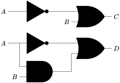
A straightforward approach is to look at the truth tables and timing diagrams.
The truth table for the top circuit shows:
| A | B | C |
|---|---|---|
| 0 | 0 | 1 |
| 0 | 1 | 1 |
| 1 | 0 | 0 |
| 1 | 1 | 1 |
The truth table for the bottom circuit shows:
| A | B | D |
|---|---|---|
| 0 | 0 | 1 |
| 0 | 1 | 1 |
| 1 | 0 | 0 |
| 1 | 1 | 1 |
The timing diagrams show:
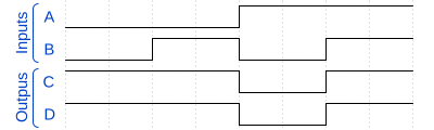
The truth tables are equivalent, and the timing diagrams match, so the circuits must be equivalent.
But this was a lot of work, and we are only comparing two inputs and outputs. There must be a better way!
The Venn Diagram#
Venn diagrams provide an intuitive, geometric way to check equivalence of Boolean expressions by treating variables as sets and Boolean operators as set operations. We use shaded areas to represent an evaluation of true, and white areas to represent an evaluation of false.
The following figure represents a constant 0; white background means the expression evaluates to false.

The following figure represents a constant 1; shading means the expression evaluates to true.

We can represent a variable with a circle. The following figure shows an interpretation of $x$. The shaded area in the circle represents an output of 1 when $x$ is true and an output of 0 when $x$ is false.
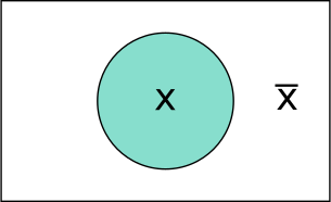
Similarly, we can evaluate $\overline{x}$ in the following figure. The diagram is the same, but now the formula evaluates to true exactly when $\overline{x}$ evaluates to true.
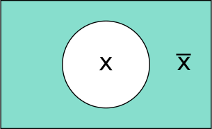
We can now represent our Boolean functions!
We use intersection ($x \cap y$) to represent $x \land y$, shown in the following figure.
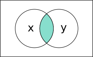
We use union ($x \cup y$) to represent $x \lor y$, shown in the following figure.
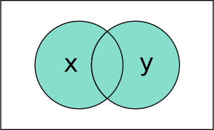
We can even evaluate more complex formulas, like exlusive or (XOR), which is true when exactly one of x or y is true, but is false when both are true.
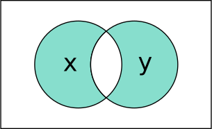
Or we can represent a formula like $x \land \lnot y$.
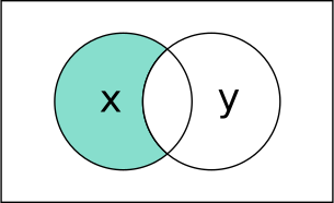
Now we have another way to check for equivalence. Two expressions are equivalent exactly when they shade the same region(s) in the Venn diagram.
How to use them in practice:
- Draw one Venn diagram that includes all variables used (two circles for two variables, three for three, etc.).
- For each expression, shade the region(s) that satisfy the expression under the above definitions.
- If the shaded regions match exactly, the expressions are equivalent.
Venn diagrams are best for small numbers of variables (2–3). They give immediate intuition about identities, complements, and distributivity. For larger expressions or many variables, use algebraic manipulations, Karnaugh maps, or canonical forms instead. We’ll discuss these in future lectures.
Discussion & Practice
As a class, let’s practice by creating some Boolean formulas and drawing their Venn diagrams.
Use resources in the textbook section 2.5.1 for additional practice with Venn diagrams.
Karnaugh Maps#
Karnaugh maps (K-maps) are a visual method for minimizing Boolean expressions by grouping adjacent minterms. They are arranged so that adjacent cells differ by only one variable (Gray code ordering). You can use K-maps to obtain minimal sum-of-products (SOP) or product-of-sums (POS) forms, which we will discuss in L9. Equivalent K-maps represent equivalent circuits.
Recipe for a Karnaugh Map#
-
Identify variables
- Count distinct variables in the formula (n). K-map size = $2^n$ cells.
- Typical layouts:
- 2 vars: 2×2
- 3 vars: 2×4
- 4 vars: 4×4
-
Convert formula to a truth table (or minterms, which we’ll discuss in L9):
- List all $2^n$ input combinations for the n variables.
- For each row, evaluate the formula and write the output (0 or 1).
- The minterms are exactly the rows that produce a 1. You can record them as:
- binary rows (e.g., 101) or
- decimal indices m0..m($2^{n−1}$) where the index is the binary value with your chosen variable order.
- Mark any “don’t-care” combinations with X (these can be used to help grouping but are not required).
- Use this table to fill the K‑map: place 1 in cells for minterms, X for don’t-cares, and 0 elsewhere.
-
Draw the grid and label rows/columns in Gray code
- Arrange row and column headers so adjacent labels differ by exactly one bit (Gray code). This ensures adjacency corresponds to single-bit changes.
- Example for 3 variables (A,B,C): use 2 rows (A=0, A=1) and 4 columns with Gray-coded BC: 00, 01, 11, 10.
-
Place values into the K‑map
- For each minterm where the formula evaluates to 1, mark the corresponding cell with
1. - Mark don’t-cares with
X(optional). - Remaining cells are 0.
- For each minterm where the formula evaluates to 1, mark the corresponding cell with
2-Variable K-Maps#
The following figure demonstrates the construction of a 2-variable K-map. On the left is a truth table, and on the right is the K-map template representing the truth table.
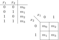
Discussion & Practice
As a class, let’s practice by creating K-maps for AND, OR, and a made-up formula
3-Variable K-Maps#
The following figure demonstrates the construction of a 3-variable K-map (usually drawn 2 rows x 4 columns in the order 00, 01, 11, 10). On the left is a truth table, and on the right is the K-map template representing the truth table. This is what lets K‑maps find groupings that eliminate variables by exploiting adjacency across map boundaries, which we will explore later.
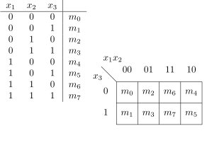
Discussion & Practice
As a class, let’s practice by creating K-maps for AND, OR, and a made-up formula
4-Variable K-Maps#
The pattern continues; see Figure 2.53 in the textbook for an example.
Discussion & Practice
As a class, let’s work through the example in Figure 2.54 of the textbook.
Algebraic Manipulation#
The above strategies are great for small circuits (2-4 inputs and 1 output), but they start to fall apart in larger networks. You’ve probably spent over a decade learning how to do algebraic manipulation to prove expressions in base 10 are equivalent. Now you’ll learn how to manipulate Boolean expressions to achieve similar proofs.
A Decimal Example#
Claim: $(x + 3)(x − 3) = x^2 − 9$.
Proof by algebraic manipulation:
- Expand using distributive property: $(x + 3)(x − 3) = x(x − 3) + 3(x − 3)$.
- Distribute inner terms: = $x^2 − 3x + 3x − 9$.
- Combine like terms $(−3x + 3x = 0): = x^2 − 9$. Thus $(x + 3)(x − 3)$ and $x^2 − 9$ are equivalent for all $x$.
Boolean Algebra#
Decimal algebra is aided by a set of theorems, such as the distributive property and the ability to combine like terms. In the next two lectures, you’ll learn theorems for Boolean algebra that will allow you to perform sophisticated analyses of Boolean expressions.
You can already do some of this manipulation yourself, working with small pieces of an expression.
Try It
As a class, prove that $x \lor (x \land y) \equiv x$